Tutorial 09: On the Hamiltonian command

The Hamiltonian command allows to compute transport by means of the NEGF formalism along a generic device defined by the user, just by simply specifying the semi-empirical tight-binding Hamiltonian in the format discussed below.
In particular, the command allows to compute the transmission coefficient as a function of the energy in the range specified by the user, and the charge density in correspondence of each atoms/grid point.
To this purpose, the hamiltonian has to be passed as a numpy bidimensional array.

The Hamiltonian to be defined is the Hamiltonian of the central part of the generic system shown below. In particular, semi-infinite leads are attached at the right and left ends of the central part, in order to compute transport within the open-boundary conditions. This is done through the definition of proper self-energies within the Hamiltonian modules (transparent for the User).

 

 

 

 

 

If the system is composed by N atoms, we can label each atom an integer (starting from 1). The first row of the Matrix specify the number of considered orbitals.

The rows 2-N+1 specify the on-site energies, while the following rows specify the hopping parameters between two adjacent atoms.

Let’s make an example in the case of one considered orbital.

The matrix will have the following form:

where E_ii represent the on-site energy for the i-th atom, while t_ij the hopping parameter between the i-th and the j-th atom.

Note that atoms ordering starts from 1 and not from 0.

The first row indicates that the model is a one-orbital model, the other rows contains information about the on-site energies of the atoms and on the hoppings between different atoms. The elements that are zero do not have to be included.
Because the hamiltonian is an hermitian matrix, only the elements on the upper part needs to be passed (i<j).

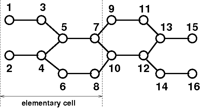
To make an example, let’s define the Hamiltonian in the above-mentioned format of the system shown in the picture below. As outlined before, the structure shown here refers to the central part of the device, while semi-infinite leads are attached at the right and left ends through the definition of the self-energies.

Within the single pz tight-binding basis set in the real space, the Hamiltonian can be expressed as follows.
In particular, we consider null on-site energies, a hopping parameter between C-C atoms equal to t=-2.7 eV, and t=-3.024 eV for the outer dimmer lines, in order to take into account edge relaxation.

The matrix to be passed reads:

1 0 0
1 1 0
2 2 0
3 3 0
4 4 0
5 5 0
6 6 0
7 7 0
8 8 0
9 9 0
10 10 0
11 11 0
12 12 0
13 13 0
14 14 0
15 15 0
16 16 0
1 3 -3.024
2 4 -2.7
3 5 -2.7
4 5 -2.7
4 6 -2.7
5 7 -2.7
6 8 -3.024
7 9 -2.7
7 10 -2.7
8 10 -2.7
9 11 -3.024
10 12 -2.7
11 13 -2.7
12 13 -2.7
12 14 -2.7
13 15 -2.7
14 16 -3.024

Please note that the matrix to be passed has to be complex, since, in generalthe hamiltonian is a complex hermitian matrix.

The definition of the matrix can be done automatically through a script, as the one you can download here. Please (rename the file with the .py extension, once downloaded).

The implemented function is called GNR, whose arguments are the number of dimmer lines N, and the number of slices M. In the example above, a python script would have read

from GNR import *
GNR(2,8)