As usual, we have first to load the NanoTCAD ViDES module:
from NanoTCAD_ViDES import *
Let us discretize a 3D domain with the following boundaries:
xmin = -1 nm, xmax = 1 nm
ymin = -2 nm, ymax = 3 nm
xmin = -10 nm, zmax = 20 nm
If we need a uniform grid, we can simply use the numpy command linspace.
For example, if we want 50 points along the x direction, 60 along the y direction
and 90 along the z direction, we simply write:
xg=linspace(-1,1,50);
yg=linspace(-2,3,60);
zg=linspace(-10,20,90);
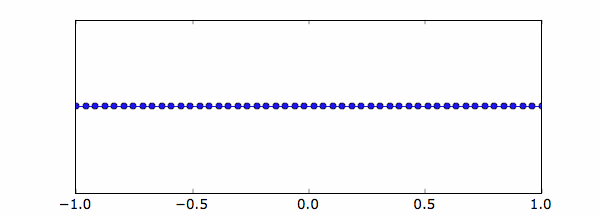
Below the uniform grid created along the x-axis
Now we can create the grid in this way:
grid=grid3D(xg,yg,zg);
In this way, all the attributes (dVe, dist, surf etc.) of the grid instance of the grid3D class are filled.
All these quantities can be handled by typing
grid.dVe
grid.dist
grid.surf
……
which are array or matrices, which one can deal as numpy array, applying all the built-in functions.
Most of the time however, it is better to deal with non uniform grids.
Let’s say for example that a non-uniform grid is need along the x direction.
We can define two regions with different mesh spacing, e.g. ∆1=0.2 and ∆2=0.05, between -1 and 0
and ∆1=0.05 and ∆2=0.2, between 0 and 1.
To do this we have to type:
xg=nonuniformgrid(array([-1,0.2,0,0.05,1,0.2]))
The results is shown here
Same considerations follow for the y and z axis.
Let us now exploit the commands explained above, in order to discretize a 3D domain, which contains a (13,0) CNT, 15 nm long. The diameter of the CNT is 1 nm, which means that the boundaries along the x and y axis are -0.5 nm and 0.5 nm. Let us consider a lateral spacing of 1 nm along the x and y directions.
As a consequence, in accordance with the position of the x,y,z axis with respect to the CNT as shown here, the limits of the 3D domain have to be set to
xmin = -1.5 nm, xmax = 1.5 nm
ymin = -1.5 nm, ymax = 1.5 nm
xmin = 0 nm, zmax = 15 nm
If a non-uniform grid wants to be used, the commands read
xg=nonuniformgrid(array([-1.5,0.2,0,0.05,1.5,0.2]))
yg=nonuniformgrid(array([-1.5,0.2,0,0.05,1.5,0.2]))
where the same grid for the x and y axis have been considered.
Equivalently one could have typed:
yg=xg;
Let’s now create the CNT, and the coordinates of the atoms
CNT=nanotube(13,15);
If we want to impose a grid point also in correspondence of the C atoms of the nanotube, we can type:
grid=grid3D(xg,yg,CNT.z,CNT.x,CNT.y,CNT.z);
In this way, grid.gridz contains only the z coordinates of CNT.
We can do the very same consideration for a GNR.
Let us consider a 6 AGNR, 10 nm long, and the same lateral spacing as in the same example as before,
as well as the same spacing in the x direction (1 nm).
We first create the GNR and its coordinates
GNR=nanoribbon(6,10);
To have a look at the maximum coordinates along the y direction, we simply type
max(GNR.y)
which is equal to 1.37 nm.
As a consequence, in accordance with the position of the x,y,z axis with respect to the GNR as shown here, the limits of the 3D domain have to be set to
xmin = -1 nm, xmax = 1 nm
ymin = -1 nm, ymax = 2.37 nm
xmin = 0 nm, zmax = 10 nm
If a non-uniform grid wants to be used, the commands read
xg=nonuniformgrid(array([-1,0.2,0,0.05,1,0.2]))
yg=nonuniformgrid(array([-1,0.2,0,0.1,1.37,0.1,2.37,0.2]))
If we want to impose a grid point also in correspondence of the C atoms of the nanoribbon, we can type:
grid=grid3D(xg,yg,GNR.z,GNR.x,GNR.y,GNR.z);
In this way, grid.gridz contains only the z coordinates of GNR.


