First of all, let’s import the NanoTCAD ViDES module
from NanoTCAD_ViDES import *
At this point, we have to create the nanoribbon. Let’s say for example we want to
study a 6 armchair GNR, 3 nm long. We can do this by typing the following command:
GNR=nanoribbon(6,3)
Note: the very same considerations works also for the class nanoribbon_fast_ohmic. Actually the only difference is that you have to change the line
GNR=nanoribbon(6,3)
with
GNR=nanoribbon_fast_ohmic(6,3)
When instancing the class nanoribbon, the method atoms_coordinates() is called and that the atoms coordinates of
the nanoribbon are computed and stored inGNR.x, GNR.y and GNR.z:
Equivalently one could have typed.
GNR.atoms_coordinates()
In partucular, the i-th C atom of the nanoribbon has the coordinates
GNR.x[i], GNR.y[i] and GNR.z[i]
Note that GNR.x is equal to zero for all the atoms. The origin is placed in the top left corner of the nanoribbon. In our notation the n-AGNR has n atoms on each unrolled ring of the nanotube. In this particular case, we have 6 atoms. Generally, in the literature, such a nanoribbon would have been called 12-AGNR.
The atoms_coordinates() function is not important for the computation of the free charge and the transmission coefficient of the nanoribbon, but it is necessary when defining the grid to be used in the self-consistent solution of the NEGF and of the Poisson equations, as it will be explained in the grid and in the self-consistent solution scheme tutorials.
In order to compute the free charge and the transmission coefficient within the real space approach, it is sufficient to run the command
GNR.charge_T()
If not specified, the potential in correspondence of each C atom is imposed to zero. Otherwise, the electrostatic potential can be imposed, by varying the GNR.Phi array.
The energy and the transmission coefficient are stored in the arrays GNR.E and GNR.T
If matplotlib module is install, the transmission coefficient can be plotted by means of the following command:
plot(GNR.E,GNR.T)
show()
The upper and the lower limit for the energy, can be specified by the user, changing the attributes Eupper and Elower of the instance GNR as shown also in the tutorial regarding the nanotube.
If not specified, Eupper and Elower are automatically computed.
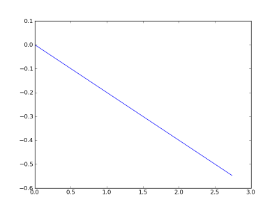
Let’s now try imposing a linear electrostatic potential along the nanoribbon, and equal to Phi(z)=-0.2*z (V)
GNR.Phi=-0.2*GNR.z
To check if the potential is exactly what we wanted, we can plot with
plot(GNR.z,GNR.Phi)
show()
Electrostatic potential (V) as a function of the z coordinates (nm)
Let us impose an electrochemical potential for the right reservoirs equal to -0.3 eV
GNR.mu2=-0.3 eV
and compute the charge and the transmission coefficient
GNR.charge_T()
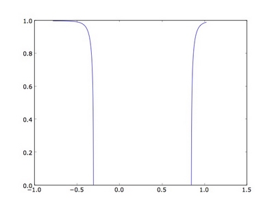
The transmission coefficient is the following:
Once done, the current can be computed and printed with
print GNR.current()


